Rainfall Statistics for Wastewater Water Balance
1. Introduction
Prior to reading this section, you need to be familiar with the page on Water Balance to understand the components of rainfall, rainfall intensity, evaporation, transpiration and evapotranspiration as these terms apply to water balance modelling.
This document "Rainfall Statistics for Wastewater Water Balance" is available for download, click on hyperlink..
"Simplified Rainfall Statistics for On-site Wastewater Management: Which Statistic Applies?" is available for download, click on hyperlink.
"Rainfall Statistics - An Exercise: Choose an appropriate statistic" is available for download, click on hyperlink.
Water balance modelling can be performed on various data sets depending upon the data available and the degree of precision provided by the modelling calculations. A water balance model is simply a number of calculations, using simple formulae, that can be performed by a computer much faster than one could do the same calculations by hand, often seconds compared with hours. The benefit of a model is that you can ‘test’ the ‘sensitivity’ of the output by varying the inputs and make a decision based upon those variables.
However, you have probably heard the expression "garbage in - garbage out" meaning that the output of the model (your assessment of the land application area required) can only ever be as good as the data selected for the model. Here lies the catch - do you have a daily time step model using all the historical rainfall recordings for your location (maybe 100 years), and the daily evaporation data, or do you use computed monthly historical rainfall and evaporation data. . Remember that rainfall is random - there is no connection with previous rainfall events to the predicted rainfall, much less what actually falls. The next 20 years may not resemble the last 20 years or any other 20 year period - that's the nature of global and local weather!
While there may be seasonal factors that influence rainfall and temperature - some areas have summer rainfall, others have wet winters, while in coastal areas rainfall may vary only slightly over all months. We know that the tropical areas have monsoon rains and cyclones in summer and the alpine areas have snow and freezing conditions in winter. All these variables impinge upon our ability to effectively return water to the hydrologic cycle without off-site discharges. In water balance modelling, we attempt to model the addition of wastewater to the normal weather conditions and landscape (rainfall, evaporation, runoff and drainage) so that at no time, given reasonable risk scenarios, does the wastewater leave the application area and present a hazard to human health or the environment. It’s that modelling that allows to adjust inputs against various combinations of outputs to develop a reasonably acceptable outcome.
A visit to the Bureau of Meteorology's website (www.bom.gov.au) will indicate that there are many statistics that could be used for water balance modelling. In the following sections we will examine some of the nonsense values we could choose (too wet or too dry distributions) and some logical statistics that provide an appropriate level of risk of failure. While we can plan for no failures of the land application area, it is probable that you could not afford such large area development and those large areas would likely not sustain vegetation during dry periods. Land application areas only work adequately when they are vegetated and if you cannot keep the plants alive in really dry times, you won't have the vegetation ready to go when it rains. Hence, minimising the risk of failure is a balance between having enough sustainable land application area most of the time. Remember, vegetation is the mechanism for return of water vapour to the atmosphere.
After reading this article, you may benefit by reading the accompanying document Simplified Rainfall Statistics for On-site Wastewater Management: Which statistic applies? The inputs to a water balance are explained.
2. Calculating Statistical Ranks
Let's start by ensuring that the statistical terms for rainfall and evaporation are the same as that used by water balance modellers and the meteorological records. Instead of writing 25th percentile, we will shorten it to 25%ile, and for all others.
Firstly, we make a list of rainfall annual values and arrange them in numerical order, the highest at the top of the list.
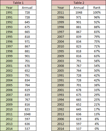 Table1
shows 25 years of annual rainfall data for Armidale NSW from 1991 to 2014,
the years listed in chronological order.
Table1
shows 25 years of annual rainfall data for Armidale NSW from 1991 to 2014,
the years listed in chronological order.
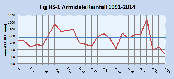
It is clear that the rainfall is highly variable over the years, more clearly illustrated in Figure RS-1 and that few consecutive years reflect the previous years, except to 1992, 1993 and 1994, and again in 2008, 2009 and 2011. We could say the totals are "all over the place" with no clear pattern. That is the random nature of the rainfall.
Because it is wet one year, (1996, has no connection to the previous year of the year following. Similarly for 2011, the s no connection with the near average rainfall of 2011 or the below average rainfall of 2012. The annual events are random. If we were to graph daily rainfall within any of the same months each year, this random nature would also be observed.
Now take the data in Table 1 and rank the rainfall (and its year) from the highest (at the top) to the lowest (at the bottom). This re-ordering by rank is easily performed in a spreadsheet simply by selecting 'data' then 'sort' in descending order)
Under the column "Rank" show the rank of each value. As there are 25 years of data, each year will have roughly a difference of 4% (100 divided by 25), with 100% at the top and 0% at the bottom, as shown in Table 2. Note that there are two annual values of 728 mm, so they are of equal rank. A facility exists within most spreadsheets to automate this ranking. In ExcelTM there are preset functions to do these calculations.
Now we can pick out the highest (100%ile), lowest (zero percentile) and the median (50%ile). We could also find the 25%ile and the 75%ile as these are clearly identified in Table 2..
What if we wanted the 60%ile? All that is shown is that the 63%ile is 816 mm and the 58%ile is 791 mm. Since there are 5%ile between the two, and 25 mm difference, divide the 25 mm by the 5 percentile rank to find that one percentile rank equals 5 mm. Therefore, to get from 58%ile(791 mm) to the 60%ile, add two times 5 mm. Therefore the 60%ile is 791 + 10 = 801 mm. The value is the same as if you took 3 x 5 mm from the 63%ile (816 - 15 = 801). So now we can find any percentile value within the 25 rainfall years above. The same method is used for any number of years of rainfall data.
3. Annual Statistical Values
Using Table 2, there are several statistics that we can develop from those 25 annual totals. Be aware that this record is only 25 years old compared to more than 150 years of records for Armidale. Only 25 years of data have been selected to make the explanation as simple as possible.
The lowest is the bottom of the list, (1%ile) the value that is exceeded ALL the time = 537 mm. Every year we can expect to get more than 537 mm rainfall (based on 25 years). If all the data since 1857 was used, then 421 mm is the lowest annual rainfall ever received.
The highest is the top of the list, (100%ile) the one that has not been exceeded in the 25 years = 1048 mm. (1508 mm in 150 years)
The difference between the smallest and the largest is 1048 - 537 = 511 mm, which we call the range.
The average annual rainfall is found by adding all 25 annual values and dividing by the number of entries (25) = 18 983 divided by 25 = 759 mm. (791 mm in 150 years)
The median value is the mid-point in the ranked list of annual values, the 50%ile = 764 mm (from Table 2). If we were to draw the average line across Figure RS-1, there would be 50% of the years above the line, and 50% below the line. Why? Because the median is the mid-way point of the ranked data - half way in the number of events, not half way between the lowest and the highest values.
Note that the average and the median are very close together, the median is slightly higher than the average. That is not always the case. For example if the top two rainfall values were 1148 and 1071 mm respectively, the average would now be 767 mm but the median would not have changed. Similarly, if the lower two values were 610 and 615 mm, the average would now be 763 mm. but there would be no change to the median. And if we changed both the top five and the bottom five there would still be no change. Why? Because the median is the mid-point of the ranked list of values, whereas the average changes as the sum changes.
The 75%ile is equalled or exceeded in only 25% of the time (all the values above 834 mm). (895 mm in 150 years)
The 25%ile is equalled or exceeded in 75% of the years (all values above 665 mm). (671 mm in 150 years)
Note: the difference between the recent 25 years and the whole data record of 150 years is relevant to our discussion. Which data set do you use?
Another way to look at these values is probability (or you may know this as 'risk'). What is the probability of getting more than 901 mm? That value is the 92%ile on Table 2. Therefore there is only an 8% chance (100%-92%) of that rainfall being exceeded. The 92% of values are all less than 901 mm.
Another statistic that is commonly used is the standard deviation, but for this exercise we are not concerned with that calculation. The common spreadsheets have specific formula to calculate this when you need it.
Which statistic we use depends upon the level of risk we are prepared to take, and the cost of meeting that risk base. Sometimes the level of minimum risk is imposed upon us by legislation when it comes to public health and/or environmental protection.
None of us has the resources (money or land application area) to have NO RISK because we are dealing with highly variable rainfall events. We have 'an acceptable risk' to work towards.
.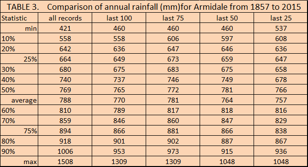
From Table 3 you can compare the difference between selecting the last 25 years' data to the other periods. From 70%ile and above, the recent 25 years' data are lower than the full record. Which period you choose will need to be justified.
4. Monthly Statistical Values
Water balance models can be run on either daily or monthly time steps. While daily modelling may allow for some period of the day to contribute to evapotranspiration, the data compilation is more arduous as the daily data over many years must be used to calculate the daily land application rate. How well future daily rainfall mimics the historical data that must be used is anyone's guess, although the longer the record, the lower the variations, perhaps!
In some locations, the long rainfall record does not always reflect the same atmospheric and location parameters. How well were recordings read and transcribed by observers? How do these recordings compare with automated values? How accurate and precise are modern pluviometers (measure rainfall intensity, rainfall with time)? Has the location of the weather station changed because of urban conditions? Is the new location subjected to different conditions to the earlier location? These are all questions we need to consider when choosing large data sets.
In this section we will examine the various monthly data options available to meet the different risk scenarios that one may encounter. Let's not be sidetracked by current government guidelines that appear to have ignored the statistical realities of using either monthly or daily time-step modelling. Bear in mind, that any risk analysis is the understanding of both the probability of a failure and the consequences of that failure. Often financial costs will need to be considered as part of the overall assessment. In wastewater risk analysis, most of the risk will be in relation to a failing system manifesting itself in some human public health or environmental harm. Mostly the risk analysis will be for perceived risk.
The NSW "Environmental Guidelines - Use of Effluent by Irrigation" (DEC, 2004) that the monthly time-step model can over-estimate the amount of wet weather storage (effluent that is excess to drainage and evapotranspiration). Hence, the general use of a monthly model is conservative. Whichever model is chosen, we are taking historical data and projecting it to represent future periods that may not mimic the past.
In Tables 1 and 2, we used only the annual data. Water balance modelling on annual data is too vague in its calculation of an appropriate land application area.. Daily time-step is just too complex for a model that is simply using typical daily values of wastewater generation and averages for evapotranspiration and seasonal crop factors, and estimates of deep drainage from estimates for soil permeability. So let's concentrate on modelling using monthly data and discuss which statistical values we use.
The rainfall records for Armidale spans the period 1857 - 2015, although the recordings were from several locations, and instrumentation has changed over that period. . The 159 years of record are used for the same process as shown in Table 2 to calculate various percentile values for each month and the annual value. These are shown in Table 4. Remember, we are seeking the monthly values that will provide a reasonably acceptable risk, not the monthly values that will give us the smallest land application area.
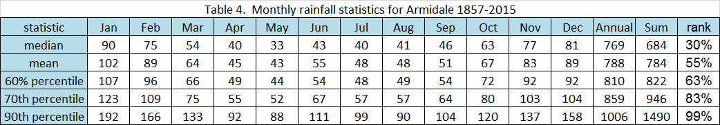
In Table 4, the monthly statistic has been calculated from all years of data (1857-2015) using the Excel in-built formulae. The 'ANNUAL' column is the actual annual total for that statistic, that is, the median annual rainfall over all records is 769 mm, and the mean rainfall is 788 mm. For the monthly water balance, the monthly totals are used for the chosen statistic which when summed is shown in column 'SUM". In the 'RANK' column, the 'SUM' has been found within the ranked annual data and shown as an equivalent percentile rank.
Let's look at the values in the row 'MEDIAN'. Each month shows the median value of the rainfall from the 159 years of data, and the 'ANNUAL' column shows the median annual total of recorded rainfall for the same 159 years. If you were to use the median data, as indicated in the NSW Guidelines, those are the values you would use in your monthly model, as set out in the 'MEDIAN' row. Unfortunately, when you 'SUM' those monthly median values you derive the value under 'SUM' column. In the case of median, the sum of the monthly totals is 684 mm but the actual median annual total was 769 mm. The 'SUM' value of 684 mm is equivalent to the 30th percentile of the actual annual totals, meaning that instead of the rainfall occurring at the mid-point of all 159 readings (that's what median means), this value of 684 mm is really only equivalent to the 30th percentile. Therefore, 70% of all annual totals are greater than 684 mm (the summed median value), so you have just designed for a failure in seven out of every 10 years. The 'MEDIAN' monthly statistic presents a high risk factor that is less than ideal and in closely settled areas would be totally unacceptable.
What that means is that the NSW Guidelines (DLG et al., 1998)seriously under-estimate the annual rainfall, for a water balance based on median monthly values, and invites failure of the system in seven out of ten years. Remember, the median value is just the mid-point in a list of ranked numbers, having nothing to do with either the highs and lows or the spread of data - just the reading that occurs at mid-point in the ranked list.
The alternative to such a high risk, as shown by choosing the 'median monthly values', is to choose some other statistic that reduces the failure of the water budget to more acceptable levels. A failure of five out of ten years is a better proposition and can be found using the 'AVERAGE' statistic. As shown in Table 4, the sum of the monthly averages is 784 mm whereas the average of the 159 years of annual rainfall totals is 788 mm. In overall terms, the AVERAGE values is equivalent to the 55th percentile - a failure of slightly less than five in every ten years.
Unfortunately, some regulators have run-riot on choosing the 'preferred' statistic. Yes, there are council that choose the 90th percentile monthly values for the water budget. Such a choice needs to be checked against actual rainfall records and examined for its applicability. Let's look again at Table 4, row headed '90th percentile'.
The 90th percentile monthly rainfall is shown under the monthly heading. The 90th percentile annual total is listed under 'ANNUAL' and has been derived from actual annual rainfall totals (1006 mm). The 'SUM' column is the total sum of the monthly columns of monthly 90th percentile values. These monthly totals are the values used in a monthly water balance that show you are using an annual rainfall of 1490 mm. That's 484 mm more than the actual 90th percentile annual value, or equivalent to the 99th percentile rainfall - just short of the wettest year in the 159 year record (1508 mm in the year 1863). Since when do we develop water balances for such high rainfall to offset an acceptable risk? Few other engineering facets of our modern cities (other than large dams or major bridges) works on such a risk analysis that it uses the data from the (near) wettest year on record.
My preference is to choose a lower risk scenario developed using the 70th percentile monthly values. Even in the case of Armidale, the 'SUM' value (946 mm) is higher than the 70th percentile 'ANNUAL' value (859 mm), mimicking the 83rd percentile, Even if I used the 60th percentile monthly values, that would be equivalent to the 63rd percentile of actual annual rainfall. Far more conservative than the median values suggested in the NSW Guidelines.
5. Monthly Statistical Values for Other Towns in NSW
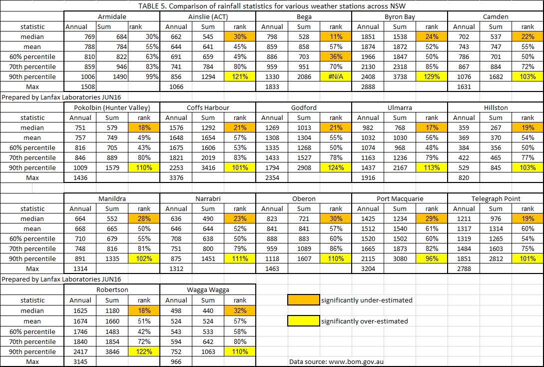
While the discussion above has been for my home town of Armidale and developed around on-site assessments and inputs into the local on-site sewage management policy of Council, the same assessment can be done for every other town in NSW, as the need arises. To assist Council regulators in better understanding the statistical realities of monthly and annual rainfall, Table 5 has been prepared for other NSW towns. In every case the use of the sum of median monthly rainfalls equates to 30% or less of the actual annual rainfall. On-site systems design on this basis have a high probability (risk) of failure. At the other end, in every case the use of the 90th percentile values is equal to or higher than the highest rainfall recorded since records began. The 90th percentile for Bega (south coast NSW) is 250 mm/year higher than the highest on record.
It is perhaps because of lack of understanding of the frequency of rainfall periods, and risk management of on-site systems, that some councils have ignored simple tools and simple statistical skills to strive for significantly over-designed land application areas. There are councils in NSW and Victoria, to my knowledge, that demand 90th percentile monthly rainfall values that provide for an annual total that is wetter than the wettest year on record for that town - unbelievable in this day and age.
6. Multi-choice method - years around 70th percentile
Where there may be some requirement for special water balance appraisal, simply repeat the water balance using six years of data around the 70th percentile rainfall to test the sensitivity of the land application area to random changes in seasonal monthly rainfall. As an example, the 159 years of data for Armidale are ranked according to their percentile value (use percentrank in Excel) from the lowest to the highest. Around the 70th percentile, choose three years below and three years above, as shown in Table 6.
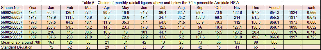
Note that 1973 and 1895 fall on either side of the 70th percentile (coloured orange), the years 1924 and 1917 are immediately below the 70th percentile while 1976 and 1997 (light green) are above the 70th percentile. Since these values are actual rainfall records, then there is no difference between the actual and the percentile sum as we saw in Table 4. The months are not ranked, only the total.
Now run the water balance for each of those six years and determine the difference the variability in rainfall makes. Notice the difference in the monthly values, while the annual rainfall, on which the data are ranked are around 860 mm, give or take a few millimetres. Armidale has a summer dominant rainfall, note the variability in summer. For these six years, January, for example has rainfall range of 60 - 256 mm, December 28-197 mm. During winter variability can also be high, June 18-101 mm and August 5-63 mm.
While you could choose the rainfall record that gave the smallest land application area, it may not be rainfall that is critical, wastewater generation may be determining factor.
Unfortunately the same cannot be done for evaporation for all towns because of the scant data available. Hence average monthly evaporation is used as a surrogate for variability. Much more work needs to be done to get a closer association between variations in rainfall, temperature and evaporation than is usually practical for a simple water balance for a single household.
7. Variability of data around 70th percentile
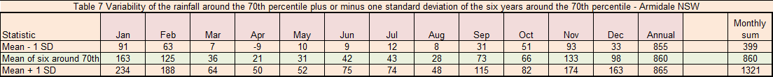
The discussion around Table 6 simply showed that the six years of recorded monthly data appeared very different across the six years. The next important observation is that the mean value of those six years is very different from the actual years. We can calculate the standard deviation (SD) and show a value for that deviation. In Table 7 the first line is the mean value minus one standard deviation, the second line the mean value and the last line the mean value plus one standard deviation as a gauge of the possible spread of rainfall values. Unfortunately, the last column "SUM" is the sum of the monthly values for that row, the variation is enormous. It would not be reasonable to test the water balance against the monthly values simply because of the great difference, but it would be reasonable to use the mean of those six years of data. We will later see how all these variables lead to variations in a water balance outcome.
8. Actual water balance outcomes
So are you confused as to which rainfall data you should use? I would think that you are because the rainfall is so unrelated from one day to the next and therefore from one year to the next. The only pattern that may become obvious is that for Armidale there is a summer dominance and a relatively dry winter. Therein lies some of the essential inputs to our water balance model. We have high evaporation and high rainfall in summer and low rainfall but very low evaporation in winter. Unless we adopt a water balance model, it would be unreasonable to simply equate the size of the land application area as suggested in Equation Q2 of AS/NZS 1547:2012 (page 181) because that equation takes no account of the monthly variability.
Let's take the water balance model that was used in Australian Standard 1547 -1994 and omitted from the updates to the Standard since then. Why? Who knows?
Inputs to model:
monthly rainfall (statistic to be chosen) minus
proportion as runoff (depends upon many factors)
monthly wastewater production - related to number of persons
Outputs from the model:
monthly evaporation (daily average times number of days) multiplied
by a crop factor (different summer to winter) to give monthly evapotranspiration
monthly drainage loss (daily loss depending upon soil
permeability time number of days)
changes in soil water storage capacity based upon porosity of the
soil. In the case of sub-soil trenches, this void space takes into account
the space in the drainage pipe or corrugated tunnel.
Scenario
Household of four persons generating 600 L wastewater per day from
reticulated water supply
(4 x 150 Lpd)
Aerated wastewater treatment system with above ground
irrigation
Land application area loam A horizon over a clay loam B
horizon - irrigation rate of 3.5 mm per day based upon clay loam
Soil porosity 40% and crop factors 0.85 Oct-Mar; 0.6 Apr-Sep.
Runoff coefficient 25%
Maximum monthly in-soil water storage (10 mm water equivalent
to 25 mm saturated soil)
Average daily evaporation - unchanged for each water balance
- set at known current daily average.
The water balance model was run for each of the six years set out in Table 6 including the mean of each monthly value. The results are tabulated in Table 8.
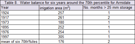
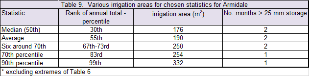
The interpretation of Table 8 shows that even when monthly values from years around the 70th percentile annual rainfall provide different land application areas. The mean of the monthly 70th percentile rainfall values gave the smallest irrigation area because it 'dumbed down' the extremes. Which irrigation area is most suited? I'd suggest that perhaps 168 m2 may be too small and 305 m2 may be too large and we need to accept some risk and go with the 250-260 m2.
At a maximum in-soil loading of only 25 mm of wet soil (10 mm of water), the system has significant capacity for more in-soil storage, possibly up to 200 mm water, and that can buffer against rainfall events that may be higher than the 70th percentile.
9. Now what is the choice of rainfall statistic?
It is easy to be confused by the choice of rainfall statistic that we can use to mimic what may happen in the years ahead because of what happened in the years gone-by. But just how reasonable those figures are depends on the sensitivity of the model as well as the rainfall pattern.
The NSW Guidelines (DLG et al., 1998) unfortunately suggest (page 159) that the median (50th percentile) monthly rainfall is the desirable statistic. As can be seen in Table 5 the median or 50th percentile monthly values only sums to be equivalent to about the 25-30th percentile of the annual rainfall; the risk of failure is seven out of every ten years. Compare those high failure years for the median to the rainfall values for the mean (average) year. Again, from Table 5, at least the average monthly values sum to about the average of the annual actual value; a much lower risk at about 50/50 than that of the median. For some towns the difference between the median and the mean rainfall is small, but large for other towns simply because of the variability of the rainfall over the recording period and their geographic location.
For those regulators who require the lowest risk and choose the 90th percentile, again Table 5 shows that the sum of the monthly 90th percentile values is mostly higher than the wettest year on record. That's not being risk averse, that's stupidity that creates significant financial burden on the home owner and the high risk of failure of an irrigation area in the dry periods as the vegetation dies from lack of water. Table 9 shows that the 90th percentile value is nearly twice the area required by the NSW Guidelines. Remember, the vegetation is the pathway for most of the water back to the atmosphere and increasing the irrigation area may be detrimental in the long run.
Now let's take the same water balance model (same variables) used in Section 7 and compare those two statistics (monthly median and monthly average) with the 70th percentile monthly values that have low risk of failure and reasonable economic value. Which statistic do you prefer because it represents a 'reasonable' risk?
10. Conclusion
The benefit of completing a water balance is that it provides some idea of the sensitivity of the constraints of the land application area (size, permeability, drainage) to the vagaries of rainfall, evapotranspiration and monthly wastewater inputs. Without a water balance, there is no understanding of how small changes to one or more variable will interact with the soil. It is not an exact science so there is a risk, but when we choose parameters that have some credibility we can minimise the risk. As seen in Table 5, when we select ridiculous rainfall statistics, we can either significantly under-estimate or significantly over-estimate the impact upon the land application area.
The other constraints of crop factors, drainage rates and horizontal movement of water pale to insignificance when the rainfall regime is wrong. When we under-estimate rainfall, the probability (risk) that the land application area will be overloaded for many months of the year is very high, with a high risk of wet and boggy land application area and possible leakage off-site. When we over-estimate the rainfall, there is also a probability that the land system will fail because the area is too large to be irrigated with effluent in the summer months and the vegetation will die. Since the vegetation is the major pathway back to the atmosphere, the land application area will fail to operate as designed - another failure.
Since a water balance is simply a calculation of 'water in' and 'water out', simplicity is the key. We cannot expect to know the actual rainfall over the next 10 years, but we can use some reasonable statistical values to derive a possible and/or probable rainfall regime. We can err on the side of caution or we can be simply blinded by the numbers. The key is 'low risk'.
There are, however, some lessons to be learned from the above. Firstly, choosing the median monthly rainfall inevitably leads to failures in the order of seven out of ten (Table 5). Choosing the 90th percentile monthly rainfalls is absurd as in nearly all cases cited in Table 5 it leads to annual rainfall values higher than has ever been received since recordings commenced. No other industry, save for the Dam Safety Committee uses these extreme statistics. The enormous cost to individual and society from a small risk of failure cannot be justified by choosing either the median or 90th percentile monthly values.
At best, the average monthly rainfall accounts for a failure five years in 10, and the 70th percentile monthly values for two years in 10.
What is more important is the gauge of sensitivity of the model to changes in rainfall, evapotranspiration, soil permeability and effluent load in determining a safe and sustainable land application area.
11. References
Bureau of Meteorology Climate Data Online access from http://www.bom.gov.au/climate/data/index.shtml
DEC (2004) Environmental Guidelines: Use of Effluent by Irrigation . Dept. Environment and Conservation, Sydney
DLG et al., (1998) NSW Environment and Health Protection Guidelines: On-site sewage management for single households NSW Dept Local Govt, NSW Environ. Protection Authority, NSW Health, NSW Land & Water Conservation and Dept Urban Affairs & Planning.
Lanfax Laboratories, accessed from www.lanfaxlabs.com.au/
Standards Australia (1994) Australian Standard AS 1547-1994 Disposal systems for effluent from domestic premises. Standards Australia. Sydney.